Available environments

This page is organized as follow:

List of available environment

How to get the up to date list

The complete list of test environments can be found using:

import grid2op
grid2op.list_available_test_env()

And the list of environment that can be downloaded is given by:

import grid2op
grid2op.list_available_remote_env()

In this case, remember that the data will be downloaded in:

import grid2op
grid2op.get_current_local_dir()

Description of some environments

The provided list has been updated early April 2021:

env name	grid size	maintenance	opponent	redisp.	storage unit
l2rpn_case14_sandbox	14 sub.	❌	❌ ️	✔️ ️	❌
l2rpn_wcci_2020	36 sub.	✔️ ️	❌ ️	✔️ ️	❌
l2rpn_neurips_2020_track1	36 sub.	✔️ ️	✔️ ️	✔️ ️	❌
l2rpn_neurips_2020_track2	118 sub.	✔️ ️	❌ ️	✔️ ️	❌
l2rpn_icaps_2021	36 sub.	✔️ ️	✔️ ️	✔️ ️	❌
l2rpn_wcci_2022	118 sub.	✔️ ️	✔️ ️	✔️ ️	✔️ ️
l2rpn_idf_2023	118 sub.	✔️ ️	✔️ ️	✔️ ️	✔️ ️
* educ_case14_redisp *	14 sub.	❌️	❌ ️ ️	✔️ ️	❌
* educ_case14_storage *	14 sub.	❌️	❌ ️	✔️ ️	✔️
* rte_case5_example *	5 sub.	❌️	❌ ️ ️	❌ ️ ️	❌
* rte_case14_opponent *	14 sub.	❌️	✔️ ️	❌ ️ ️	❌
* rte_case14_realistic *	14 sub.	❌️	❌ ️ ️	✔️ ️	❌
* rte_case14_redisp *	14 sub.	❌️	❌ ️ ️	✔️ ️	❌
* rte_case14_test *	14 sub.	❌️	❌ ️ ️	❌ ️ ️	❌
* rte_case118_example *	118 sub.	❌️	❌ ️	✔️ ️	❌

To create regular environment, you can do:

import grid2op
env_name = ... # for example "educ_case14_redisp" or "l2rpn_wcci_2020"
env = grid2op.make(env_name)

The first time an environment is called, the data for this environment will be downloaded from the internet. Make sure to have an internet connection where you can access https website (such as https://github.com ). Afterwards, the data are stored on your computer and you won’t need to download it again.

Warning

Some environment have different names. The only difference in this case will be the suffixes “_large” or “_small” appended to them.

This is because we release different version of them. The “basic” version are for testing purpose, the “_small” are for making standard experiment. This should be enough with most use-case including training RL agent.

And you have some “_large” dataset for larger studies. The use of “large” dataset is not recommended. It can create way more problem than it solves (for example, you can fit a small dataset entirely in memory of most computers, and having that, you can benefit from better performances - your agent will be able to perform more steps per seconds. See Optimize the data pipeline for more information). These datasets were released to address some really specific use in case were “overfitting” were encounter, we are still unsure about their usefulness even in this case.

This is the case for “l2rpn_neurips_2020_track1” and “l2rpn_neurips_2020_track2”. To create them, you need to do env = grid2op.make(“l2rpn_neurips_2020_track1_small”) or env = grid2op.make(“l2rpn_neurips_2020_track2_small”)

So to create both the environment, we recommend:

import grid2op
env_name = "l2rpn_neurips_2020_track1_small"  # or "l2rpn_neurips_2020_track2_small"
env = grid2op.make(env_name)

Warning

Environment with * are reserved for testing / education purpose only. We do not recommend to perform extensive studies with them as they contain only little data.

For these testing environments (the one with * around them in the above list):

import grid2op
env_name = ... # for example "l2rpn_case14_sandbox" or "educ_case14_storage"
env = grid2op.make(env_name, test=True)

Note

More information about each environment is provided in each of the sub section below (one sub section per environment)

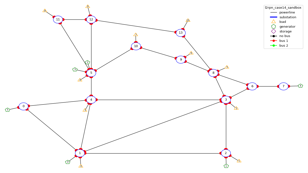
l2rpn_case14_sandbox

This dataset uses the IEEE case14 powergrid slightly modified (a few generators have been added).

It counts 14 substations, 20 lines, 6 generators and 11 loads. It does not count any storage unit.

We recommend to use this dataset when you want to get familiar with grid2op, with powergrid modeling or RL. It is a rather small environment where you can understand and actually see what is happening.

This grid looks like:

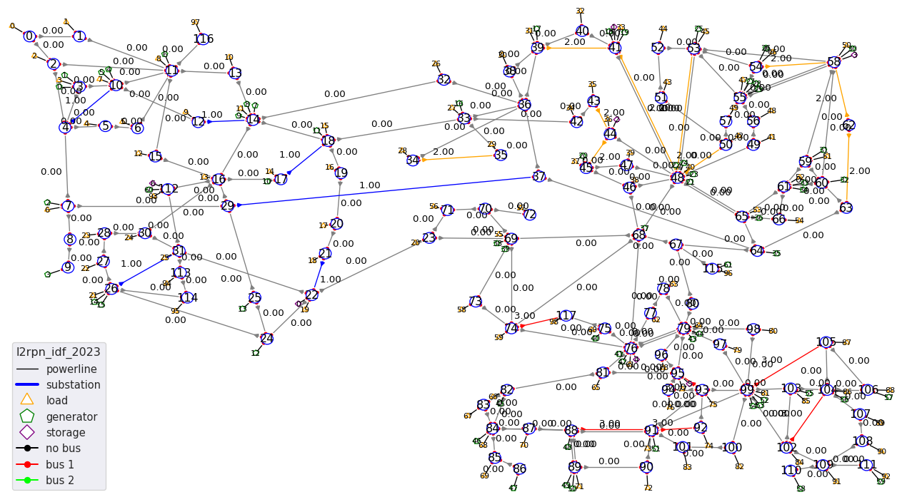
l2rpn_idf_2023

This environment is also based on the 118 grid. The original grid has been modified (mainly for generator and loads location) to accomodate for the “possible energy mix” of France in 2035.

It comes with 16 years worth of data, 1 year being divided in 52 weeks so 16 x 52 = 832 different scenarios and takes up around ~ 5.4 GB of space.

To create it you can :

import grid2op
env_name  = "lrpn_idf_2023"
env = grid2op.make(env_name)

It counts 118 substations, 186 powerlines, 99 loads and 62 generators. It will be used for the L2RPN competitions funded by Region Ile De France: “Paris Region AI Challenge Energy Transition” and is free to use for everyone.

You have the possibility, provided that you installed chronix2grid (with pip install grid2op[chronix2grid]), to generate as much data as you want with the grid2op.Environment.Environment.generate_data() function. See its documentation for more information.

The environment can be seen:

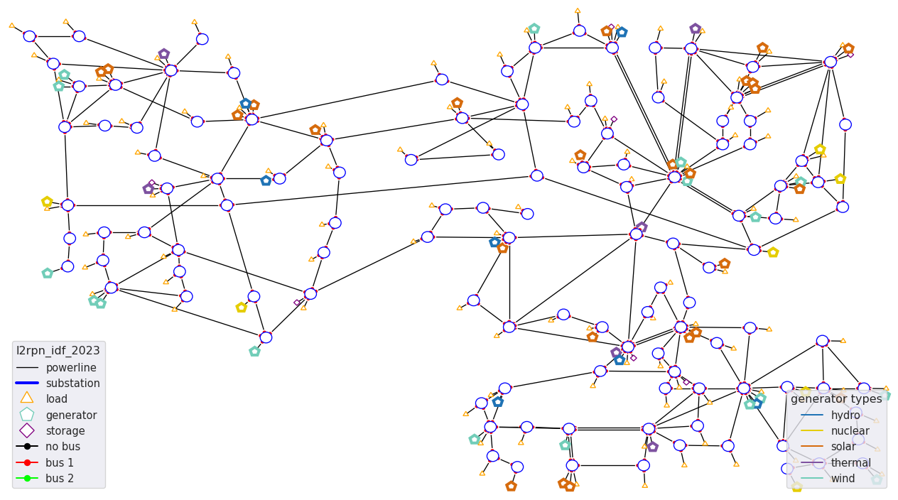
Compared to previous available environments there are some new features including:

• 12 steps ahead forecast: with any observation, you can now have access to forecast 12 steps ahead with, for example obs.simulate(…, time_step=12) or obs.get_forecast_env() which has a maximum duration of 12 steps (previously it was only 1 step ahead forecast). This could be used in model based strategy for example (see page Model Based / Planning methods for more examples)

• a more complex opponent: the opponent can attack 3 lines in 3 different areas of the grid at the same time (instead of being limited to just 1 attack)

• more complex rules: in this environment to balance for the fact that the opponent can makes 3 attacks, the agent can also act on 3 different powerlines and 3 different substation per step (one per area).

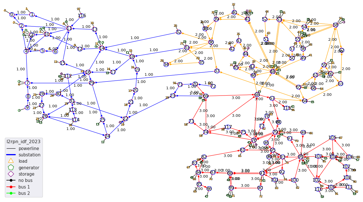
The grid is split in 3 disctinct areas:

Like most grid2op environment, it also has maintenance. Lines that can be in maintenance are:

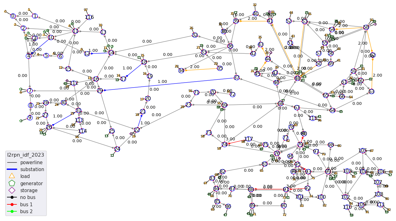
And the lines that can be attacked by the opponent are:

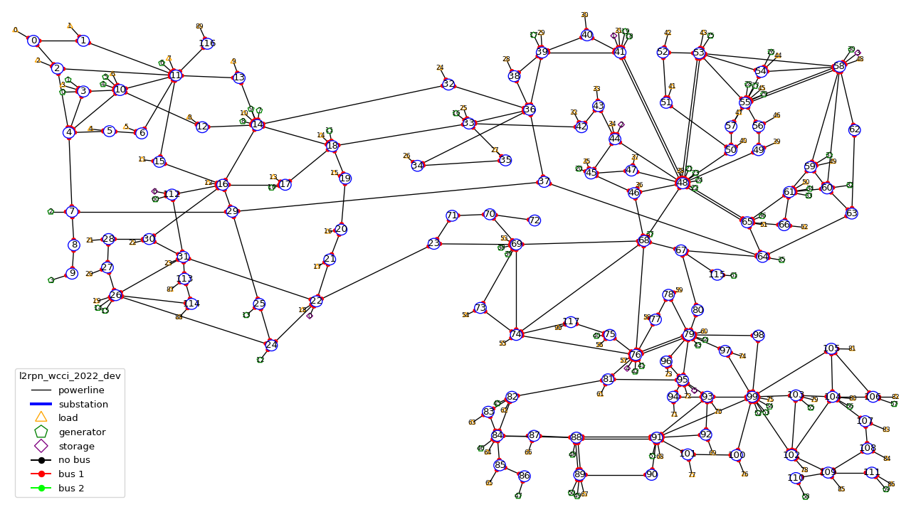
l2rpn_wcci_2022

This environment will come in two “variations”:

• l2rpn_wcci_2022_dev: development version (might not be totally finished at time of writing), to be used for test only, only a few snapshots are available.

• l2rpn_wcci_2022 : (equivalent of 32 years of powergrid data at 5 mins interval) weights ~1.7 GB

You have the possibility, provided that you installed chronix2grid (with pip install grid2op[chronix2grid]), to generate as much data as you want with the grid2op.Environment.Environment.generate_data() function. See its documentation for more information.

import grid2op
env_name  = "l2rpn_wcci_2022"
env = grid2op.make(env_name)

It counts 118 substations, 186 powerlines, 91 loads and 62 generators. It will be used for the L2RPN competitions at WCCI in 2022.

You can add as many chronics as you want to this environment with the code:

import grid2op
env_name  = "l2rpn_wcci_2022"
env = grid2op.make(env_name)

nb_year = 1 # or any postive integer
env.generate_data(nb_year=nb_year)

It might take a while (so we advise you to get a nice cup of tea, coffee or anything) and will only work if you installed chronix2grid package.

l2rpn_icaps_2021

This environment comes in 3 different “variations” (depending on the number of chronics available):

• l2rpn_icaps_2021_small (1 GB equivalent of 50 years of powergrid data at 5 mins interval, so 4 838 400 different steps !)

• l2rpn_icaps_2021_large (4.8 GB equivalent of ~250 years of powergrid data at 5 mins interval, so 23 804 928 different steps !)

• l2rpn_icaps_2021 (use it for test only, only a few snapshots are available)

We recommend to create this environment with:

import grid2op
env_name  = "l2rpn_icaps_2021_small"
env = grid2op.make(env_name)

It is based on the same powergrid as the l2rpn_neurips_2020_track1 environment and was used for the L2RPN ICAPS 2021 competition. It counts 36 substations, 59 powerlines, 22 generators and 37 loads (some of which represents interconnection with another grid).

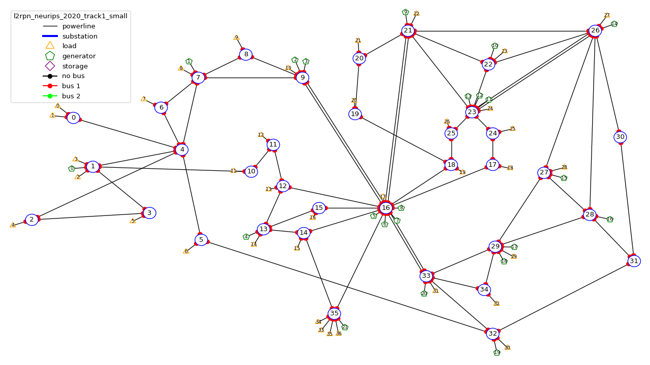
l2rpn_neurips_2020_track1

This environment comes in 3 different “variations” (depending on the number of chronics available):

• l2rpn_neurips_2020_track1_small (900 MB, equivalent of 48 years of powergrid data at 5 mins interval, so 4 644 864 different steps !)

• l2rpn_neurips_2020_track1_large (4.5 GB, equivalent of 240 years of powergrid data at 5 mins interval, so 23 22 4320 different steps.)

• l2rpn_neurips_2020_track1 (use it for test only, only a few snapshots are available)

We recommend to create this environment with:

import grid2op
env_name  = "l2rpn_neurips_2020_track1_small"
env = grid2op.make(env_name)

It was the environment used as a training set of the neurips 2020 “L2RPN” competition, for the “robustness” track, see https://competitions.codalab.org/competitions/25426 .

This environment is part of the IEEE 118 grid, where some generators have been added. It counts 36 substations, 59 powerlines, 22 generators and 37 loads (some of which represents interconnection with another grid). The grid is represented in the figure below:

One of the specificity of this grid is that it is actually a subset of a bigger grid. Actually, it represents the grid “circled” in red in the figure below:

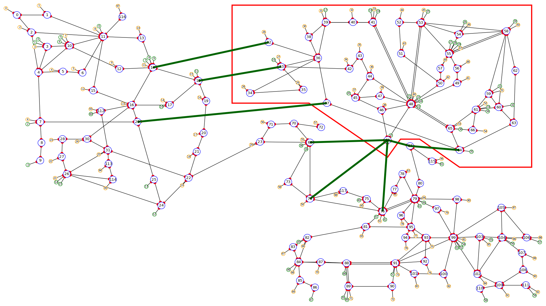
This explains why there can be some “negative loads” in this environment. Indeed, this loads represent interconnection with other part of the original grid (emphasize in green in the figure above).

l2rpn_neurips_2020_track2

• l2rpn_neurips_2020_track2_small (2.5 GB, split into 5 different sub-environment - each being generated from slightly different distribution - with 10 years for each sub-environment. This makes, for each sub-environment 1 051 200 steps, so 5 256 000 different steps in total)

• l2rpn_neurips_2020_track2_large (12 GB, again split into 5 different sub-environment. It is 5 times as large as the “small” one. So it counts 26 280 000 different steps. Each containing all the information of all productions and all loads. This is a lot of data)

• l2rpn_neurips_2020_track2 (use it for test only, only a few snapshots are available)

We recommend to create this environment with:

import grid2op
env_name  = "l2rpn_neurips_2020_track2_small"
env = grid2op.make(env_name)

It was the environment used as a training set of the neurips 2020 “L2RPN” competition, for the “robustness” track, see https://competitions.codalab.org/competitions/25427 .

This environment is the IEEE 118 grid, where some generators have been added. It counts 118 substations, 186 powerlines, 62 generators and 99 loads. The grid is represented in the figure below:

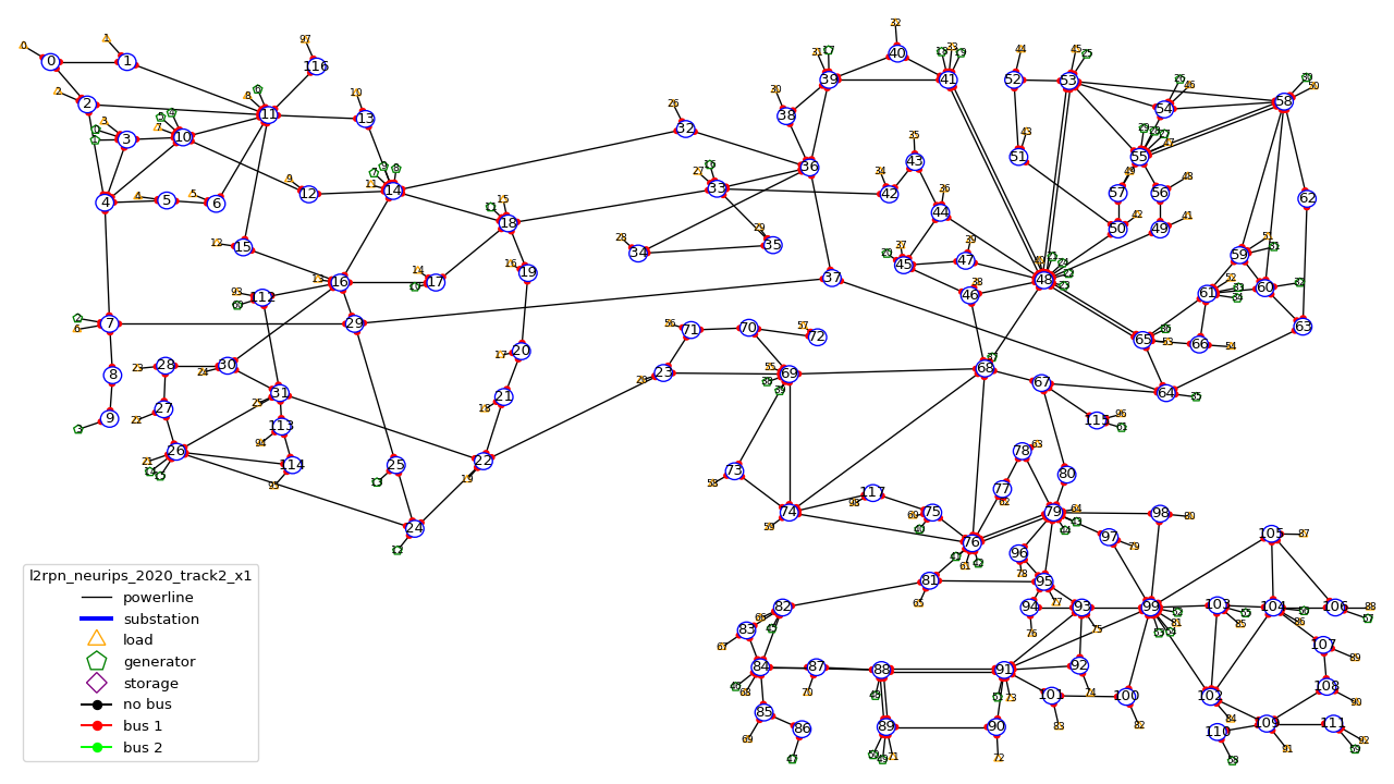
This grid is, as specified in the previous paragraph, a “super set” of the grid used in the other track. It does not count any “interconnection” with other types of grid.

l2rpn_wcci_2020

This environment l2rpn_wcci_2020 weight 4.5 GB, representing 240 equivalent years of data at 5 mins resolution, so 25 228 800 different steps. Unfortunately, you can only download the full dataset.

We recommend to create this environment with:

import grid2op
env_name  = "l2rpn_wcci_2020"
env = grid2op.make(env_name)

It was the environment used as a training set of the WII 2020 “L2RPN” competition see https://competitions.codalab.org/competitions/24902 .

This environment is part of the IEEE 118 grid, where some generators have been added. It counts 36 substations, 59 powerlines, 22 generators and 37 loads. The grid is represented in the figure below:

Note

It is an earlier version than the l2rpn_neurips_2020_track1. In the l2rpn_wcci_2020 it is not easy to identify which loads are “real” loads, and which are “interconnection” for example.

Also, the names of some elements (substations, loads, lines, or generators) are different. In the l2rpn_neurips_2020_track1 the names match the one in l2rpn_neurips_2020_track2 which is not the case in l2rpn_wcci_2020 which make it less obvious that is a subgrid of the IEEE 118.

educ_case14_redisp (test only)

It is the same kind of data as the “l2rpn_case14_sandbox” (see above). It counts simply less data and allows less different type of actions for easier “access”. It do not require to dive deep into grid2op to use this environment.

We recommend to create this environment with:

import grid2op
env_name  = "educ_case14_redisp"
env = grid2op.make(env_name, test=True)

educ_case14_storage (test only)

Uses the same type of actions as the grid above (“educ_case14_redisp”) but counts 2 storage units. The grid on which it is based is also the IEEE case 14 but with 2 additional storage unit.

We recommend to create this environment with:

import grid2op
env_name  = "educ_case14_storage"
env = grid2op.make(env_name, test=True)

rte_case5_example (test only)

Warning

We dont’ recommend to create this environment at all, unles you want to perform some specific dedicated tests.

A custom made environment, totally fictive, not representative of anything, mainly develop for internal tests and for super easy representation.

The grid on which it is based has absolutely no “good properties” and is “mainly random” and is not calibrated to be representative of anything, especially not of a real powergrid. Use at your own risk.

other environments (test only)

Some other test environments are available:

• “rte_case14_realistic”

• “rte_case14_redisp”

• “rte_case14_test”

• “rte_case118_example”

Warning

We don’t recommend to create any of these environments at all, unless you want to perform some specific dedicated tests.

This is why we don’t detail them in this documentation.

Content of an environment

A grid2op “environment” is represented as a folder on your computer. There is one folder for each environment.

Inside each folder / environment there are a few files (as of writing):

• “grid.json” (a file): it is the file that describe the powergrid and that can be read by the default backend. It is today mandatory, but we could imagine a file in a different format. Note that in this case, this environment will not be compatible with the default backend.

• “config.py” (a file): this file is imported when the environment is loaded. It is used to parametrize the way the environment is made. It should define a “config” variable. This “config” is dictionary that is used to initialize the environment. They key should be variable names. See example of such “config.py” file in provided environment.

It can of course contain other information, among them:

• “chronics” (a folder) [recommended]: this folder contains the information to generate the production / loads at each steps. It can itself contain multiple folder, depending on the grid2op.Chronics.GridValue class used. In most available environment, the class grid2op.Chronics.Multifolder is used. This folder is optional, though it is present in most grid2op environment provided by default.

• “grid_layout.json” (a file) [recommended]: gives, for each substation its coordinate (x,y) when plotted. It is optional, but we strongly encourage to have such. Otherwise, some tools might not work (including all the tool to represent it, such as the renderer (env.render), the EpisodeReplay or even some other dependency package, such as Grid2Viz).

• “prods_charac.csv” (file): [see grid2op.Backend.Backend.load_redispacthing_data() for a description of this file] This contains all the information related to “ramps”, “pmin / pmax”, etc. This file is optional (grid2op can perfectly run without it). However, if absent, then the classes grid2op.Space.GridObjects.redispatching_unit_commitment_availble will be set to False thus preventing the use of some feature that requires it (for example redispatching or curtailment)

• “storage_units_charac.csv” (file): [see grid2op.Backend.Backend.load_storage_data() for a description of this file] This file is used for a description of the storage units. It is a description of the storage units needed by grid2op. This is optional if you don’t have any storage units on the grid but required if there are (otherwise a BackendError will be raised).

• “difficulty_levels.json” (file): This file is useful is you want to define different “difficulty” for your environment. It should be a valid json with keys being difficulty levels (“0” for easiest to “1”, “2”, “3”, “4”, “5” , …, “10”, …, “100”, … or “competition” for the hardest / closest to reality difficulty).

And this is it for default environment.

You can highly customize everything. Only the “config.py” file is really mandatory:

• if you don’t care about your environment to run on the default “Backend”, you can get rid of the “grid.json” file. In that case you will have to use the “keyword argument” “backend=…” when you create your environment (e.g env = grid2op.make(…, backend=…) ) This is totally possible with grid2op and causes absolutely no issues.

• if you code another grid2op.Chronics.GridValue class, you can totally get rid of the “chronics” repository if you want to. In that case, you will need to either provide “chronics_class=…” in the config.py file, or initialize with env = grid2op.make(…, chronics_class=…)

• if your grid data format contains enough information for grid2op to initialize the redispatching and / or storage data then you can freely use it and override the grid2op.Backend.Backend.load_redispacthing_data() or grid2op.Backend.Backend.load_storage_data() and read if from the grid file without any issues at all.